Leapfrog is Symplectic for the Harmonic Oscillator
Microcanonical molecular dynamics describes the motion of molecules using the Hamiltonian mechanics framework. Hamiltonian dynamics are symplectic, meaning that they preserve volume in phase space. The symplectic property relates to properties we learned in first-semeter college physics such as conservation of energy.
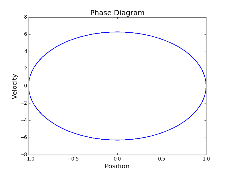
The harmonic oscillator is a simple symplectic model, useful for study. A plot of the path through phase space of our analytical derivation of the harmonic oscillator, demonstrates the symplectic property:
Symplectic integrators are important for bounding errors in the trajectories and resulting statistics such as transition rates1. Ge and Mardsen showed that if an integrator is symplectic, then the integrator can only conserve energy exactly if it computes the exact trajectory except for a reparameterization in time. Since the error in the energy is bounded, the error of statistics calculated from trajectories are bounded.
The bound would seem to contradict our results from the analyses of the local and global truncation errors. These analyses indicate that the errors in energy and other statistics computed from the trajectories would grow without bound. It turns out that symplectic integrators exactly simulate shadow Hamiltonians, which are perturbations of the original Hamiltonians. Thus, we can use the energy and other statistics from the shadow Hamiltonian as approximations to the values for the true Hamiltonian.
Additionally, the relationship between the bounds on the errors in the energy and the trajectories implies that the error in energy can be used as a measure of error for the trajectories. For example, unbounded inncreases or decreases in the energy from a simulation are indicative of an incorrect implementation of a symplectic integrator.
Unfortunately, the mathematical definition of the symplectic property and its relation to properties like the conservation of energy are expressed using advanced areas of math such as differential geometry. Fortunately, it is much easier to prove that an integrator is symplectic than it is to state the definition of symplectiness.
Hamiltonian Dynamics
We’re going to start with a detour. Symplectiness is described using the language of Hamiltonians and flows, so we’ll describe some basics and show how Hamiltonians relate to Newton’s equations of motion.
The Hamiltonian is a function that takes the positions \(q\) and momenta \(p\). The form of the Hamiltonian commonly used in molecular dynamics is a linear combination of the kinetic and potential energies:
\[H(q, p) = \frac{1}{2}p^T M^{-1} p + U(q)\]We can describe the dynamics of the Hamiltonian system using a pair of first-order differential equations:
\[\frac{dq}{dt} = \frac{dH}{dp} = M^{-1} p \\ \frac{dp}{dt} = -\frac{dH}{dq} = -\nabla U(q) \\\]The system of two first-order ODEs can be rewritten as a single second-order ODE:
\[\frac{d^2 q}{dt^2} = \frac{d}{dt} \frac{dq}{dt} \\ = \frac{d}{dt} M^{-1} p \\ = M^{-1} \frac{dp}{dt} \\ = M^{-1} (-\nabla U(q)) \\ = - M^{-1} \nabla U(q)\]By re-arranging the mass term, we get the form of Newton’s equations of motions we expect:
\[M \frac{d^2 q}{dt^2} = - \nabla U(q)\]Thus, the Hamiltonian system is an equivalent description to Newton’s equations of motion.
Symplectic Maps / Dynamical Systems
We can define a map \(\phi\) that updates the state of the system over a length of time \(\Delta t\):
\[(q_{i+1}, p_{i+1}) = \phi (q_i, p_i)\]Let \(\phi'\) be the Jacobian matrix of \(\phi\):
\[\phi' = \begin{pmatrix} \frac{\partial \phi}{\partial q} & \frac{\partial \phi}{\partial p} \end{pmatrix}\]The map \(\phi\) is symplectic if its Jacobian \(\phi'\) satifies:
\[\phi'^T J \phi' = J\]where
\[J = \begin{pmatrix} 0 & 1 \\ -1 & 0 \end{pmatrix}\]Harmonic Oscillator is Symplectic
We now have the basic tools for describing Hamiltonian systems and proving symplecticness. Let’s apply these tools. As a Hamiltonian system, the map for the harmonic oscillator is symplectic. To demonstrate the proof of symplectiness for map, we will start by validating the analytical map for the harmonic oscillator is symplectic. The Hamiltonian is defined as follows:
\[H(q, p) = \frac{1}{2}p^T M^{-1} p + \frac{1}{2} M \omega^2 q^2\]The corresponding map for the system is given by
\[\phi(q, p) = \begin{pmatrix} \cos(\Delta t) q + \sin(\Delta t)p \\ -\sin(\Delta t) q + \cos(\Delta t)p \end{pmatrix}\]with Jacobian
\[\phi'(q, p) = \begin{pmatrix} \frac{\partial \phi}{\partial q} & \frac{\partial \phi}{\partial p} \end{pmatrix} \\ = \begin{pmatrix} \cos (\Delta t) & \sin (\Delta t) \\ -\sin (\Delta t) & \cos (\Delta t) \end{pmatrix}\]With a bit of arithmetic, we see that the map satisfies the criteria for symplectiness:
\[\phi'^T J \phi' = \begin{pmatrix} \cos (\Delta t) & -\sin (\Delta t) \\ \sin (\Delta t) & \cos (\Delta t) \end{pmatrix} \begin{pmatrix} 0 & 1 \\ -1 & 0 \end{pmatrix} \begin{pmatrix} \cos (\Delta t) & \sin (\Delta t) \\ -\sin (\Delta t) & \cos (\Delta t) \end{pmatrix} \\ = \begin{pmatrix} \sin (\Delta t) & \cos (\Delta t)\\ -\cos (\Delta t) & \sin (\Delta t) \end{pmatrix} \begin{pmatrix} \cos (\Delta t) & \sin (\Delta t) \\ -\sin (\Delta t) & \cos (\Delta t) \end{pmatrix} \\ = \begin{pmatrix} \cos (\Delta t)\sin (\Delta t) - \cos (\Delta t)\sin (\Delta t) & \sin^2 (\Delta t) + \cos^2 (\Delta t) \\ -[\cos^2 (\Delta t) + \sin^2 (\Delta t)] & - \sin (\Delta t)\cos (\Delta t) + \cos (\Delta t)\sin (\Delta t) \end{pmatrix} \\ = \begin{pmatrix} 0 & 1 \\ -1 & 0 \end{pmatrix} \\ = J\]Thus, the analytical harmonic oscillator map satisfies the conditions for symplectiness as expected.
Leapfrog for Harmonic Oscillator
Next, we will prove that the Leapfrog method is symplectic for the harmonic oscillator system.
In our previous blog post, we derived the Leapfrog integrator. We reproduce it here, with the substitutions \(x = q\) and \(v = M^{-1} p\) to be consistent with the notation used in this blog post. We’ll re-arrange the integrator into two equations, one for \(q(t + \Delta t)\) and another for \(p(t + \Delta t)\), so that we can form the flow equation \(\phi(q, p)\). We will then use the Jacobian \(\phi'\) to prove that the Leapfrog integrator is symplectic.
\[F(t) = -\nabla U(q(t)) \\ q(t + \Delta t) = q(t) + M^{-1}p(t)\Delta t + \frac{1}{2}M^{-1}F(t)\Delta t^2 \\ F(t + \Delta t) = -\nabla U(q(t + \Delta t)) \\ p(t + \Delta t) = p(t) + \frac{1}{2} [F(t) + F(t + \Delta t)] \Delta t \\\]We substitute the potential
\[U(q) = \frac{1}{2} M \omega^2 q^2\]into \(F(t)\) and \(F(t + \Delta t)\) of the integrator equations:
\[F(t) = -M \omega^2 q(t) \\ q(t + \Delta t) = q(t) + M^{-1}p(t)\Delta t + \frac{1}{2}M^{-1} F(t)\Delta t^2 \\ F(t + \Delta t) = -M \omega^2 (q(t + \Delta t)) \\ p(t + \Delta t) = p(t) + \frac{1}{2} [F(t) + F(t + \Delta t)] \Delta t \\\]We substitute \(F(t)\) and \(F(t + \Delta t)\) into \(q(t + \Delta t)\) and \(p(t + \Delta t)\), reducing our system to two equations:
\[q(t + \Delta t) = q(t) + M^{-1}p(t)\Delta t - \frac{1}{2}\omega^2 q(t) \Delta t^2 \\ p(t + \Delta t) = p(t) + \frac{1}{2} [-M \omega^2 q(t) - M \omega^2 q(t + \Delta t)] \Delta t\]We substitute \(q(t + \Delta t)\) into \(p(t + \Delta t)\) to get \(q(t + \Delta t)\) and \(p(t + \Delta t)\) in terms of \(q(t)\) and \(p(t)\) only:
\[q(t + \Delta t) = q(t) + M^{-1}p(t)\Delta t - \frac{1}{2}\omega^2 q(t) \Delta t^2 \\ p(t + \Delta t) = p(t) + \frac{1}{2} [-M \omega^2 q(t) - M \omega^2 [q(t) + M^{-1}p(t)\Delta t - \frac{1}{2}\omega^2 q(t) \Delta t^2]] \Delta t\]Thus, we can form the flow \(\tilde{\phi}'(q, p)\) as
\[\tilde{\phi}'(q, p) = \begin{pmatrix} (1 - \frac{1}{2} \omega^2 \Delta t^2) q(t) + M^{-1}\Delta t \, p(t) \\ (- M \omega^2 \Delta t + \frac{1}{4} M \omega^4 \Delta t^3) q(t) + (1 - \frac{1}{2} \omega^2 \Delta t^2) p(t) \end{pmatrix}\]with Jacobian
\[\tilde{\phi}' = \begin{pmatrix} a & b \\ c & d \end{pmatrix}\]where
\[a = d = 1 - \frac{1}{2} \omega^2 \Delta t^2 \\ b = M^{-1} \Delta t \\ c = - M \omega^2 \Delta t + \frac{1}{4} M \omega^4 \Delta t^3\]Note that we denote the map as \(\tilde{\phi}(q, p)\) since it is an approximation to the true flow \(\phi(q, p)\). We then substitute the Jacobian \(\tilde{\phi}'(q, p)\) into the equation for the conditions of symplectiness and solve:
\[\tilde{\phi}'^T J \tilde{\phi}' = \begin{pmatrix} a & c \\ b & d \end{pmatrix} \begin{pmatrix} 0 & 1 \\ -1 & 0 \end{pmatrix} \begin{pmatrix} a & b \\ c & d \end{pmatrix} \\ = \begin{pmatrix} -c & a \\ -d & b \end{pmatrix} \begin{pmatrix} a & b \\ c & d \end{pmatrix} \\ = \begin{pmatrix} -ca + ac & -cb + ad \\ -da + bc & -db + bd \end{pmatrix} \\ = \begin{pmatrix} 0 & -cb + ad \\ -da + bc & 0 \end{pmatrix} \\ = \begin{pmatrix} 0 & 1 \\ -1 & 0 \end{pmatrix} \\ = J\]where
\[-da + bc = -(1 - \frac{1}{2} \omega^2 \Delta t^2)(1 - \frac{1}{2} \omega^2 \Delta t^2) + M^{-1}\Delta t( - M \omega^2 \Delta t + \frac{1}{4} M \omega^4 \Delta t^3) \\ = -1 + \frac{1}{2} \omega^2 \Delta t^2 + \frac{1}{2} \omega^2 \Delta t^2 - \frac{1}{4} \omega^4 \Delta t^4 - \omega^2 \Delta t^2 + \frac{1}{4} \omega^4 \Delta t^4 \\ = -1\]and
\[-cb + ad = -( - M \omega^2 \Delta t + \frac{1}{4} M \omega^4 \Delta t^3) M^{-1}\Delta t + (1 - \frac{1}{2} \omega^2 \Delta t^2)(1 - \frac{1}{2} \omega^2 \Delta t^2) \\ = \omega^2 \Delta t^2 - \frac{1}{4} \omega^4 \Delta t^4 + 1 - \frac{1}{2} \omega^2 \Delta t^2 - \frac{1}{2} \omega^2 \Delta t^2 + \frac{1}{4} \omega^4 \Delta t^4 \\ = 1\]Thus, the Leapfrog method is symplectic for the harmonic oscillator system.
Conclusion
In this blog post, we covered the basics of symplectic Hamiltonians and maps. We described concepts and notation from Hamiltonian dynamics and showed how they relate to the second-order differential equations used for Newton’s equations of motion. We then discussed the conditions for proving a map is symplectic.
We then applied the framework to two problems. First, we demonstrated the approach by proving that the harmonic oscillator is symplectic. Next, we showed that the Leapfrog integrator, which is an approximate map, is symplectic for the harmonic oscillator.
We covered a lot of material, but we have even more to cover in the future. First and foremost, we want to prove that the Leapfrog method is symplectic for all Hamiltonians, or at least those of the form we use in molecular dynamics. We also want to dive into differential geometry and better understand the definition for symplectiness and the relationship with the conditions we expressed above.
We also want to better understand the implications of symplectiness for simulation. In particular, we mentioned that symplectiness guarantees a bound on the error in energies and other statistics computed from the resulting trajectories. We want to better understand this relationship and examine the proofs around the relationships.
1: I’ve used papers by Donnelly and Rogers, Leimkuhler, Reich, and Skeel, Sanz-Serna, Skeel, and Yoshida as guides for this blog post.