Harmonic Oscillator
I want to start exploring numerical integrators for differential equations and how the accuracy of various methods impacts the quantities measures from the resulting simulations. Many of the differential equations that arise in physics do not have known analytical solutions; numerical integration is the only way of simulating these systems.
My particular background is in molecular dynamics (MD). MD has its own unique requirements with a wide array of techniques used to evaluate the quality of a particular integrator. It can be easier, however, to evaluate integrators using a simple model with a known analytical solution before studying more complex models. As such, I’ll be using it to experiment with integrators and analyses I find in papers. Here, I want to describe the harmonic oscillator and some of its properties.
The potential energy function of the harmonic oscillator is given by:
\[U(x) = \frac{1}{2} m \omega^2 x^2\]where \(U\) is the potential energy, \(x\) is the position, \(m\) is the mass, \(\omega\) is the angular frequency.
We will simulate the harmonic oscillator in the microcanonical ensemble. This is the formulation seen in a first-year physics class where the total energy (potential plus kinetic) of the system is conserved. The dynamics are captured in the following second-order ordinary differential equation, otherwise known as Newton’s equations of motion:
\[m\frac{d^2 x}{dt^2} = - m \omega^2 x\]The ordinary differential equation has two initial conditions: \(x(0)\) and \(v(0)\).
The analytical solution of the ODE is given by:
\[x(t) = A m \cos(\omega t + \phi)\]where \(A\) is the amplitude of the oscillations, \(t\) is the time, and \(\phi\) is the phase.
We can verify the solution by taking its derivatives
\[\frac{dx}{dt} = - A m \omega \sin(\omega t + \phi) \\ \frac{d^2x}{dt^2} = - A m \omega^2 \cos(\omega t + \phi)\]and substituting back into the ODE:
\[m\frac{d^2 x}{dt^2} = - m \omega^2 x \\ m [- A m \omega^2 \cos(\omega t + \phi) ] = - m \omega^2 A m \cos(\omega t + \phi) \\ 1 = 1\]Using the equations for the position \(x(t)\) and and velocity \(\frac{dx}{dt}\) and our initial conditions (\(x(0)\) and \(v(0)\), we can derive a system of equations for \(A\) and \(\phi\) and solve:
\[A = x(0) m^{-1} \cos^{-1}(\phi)\] \[v(0) = - A \omega^2 m \sin(\phi) \\ v(0) = - x(0) m^{-1} \cos^{-1}(\phi) m \omega^2 \sin(\phi) \\ \frac{v(0)}{x(0)} = - \omega^2 \frac{\sin(\phi)}{\cos(\phi)} \\ \frac{v(0)}{x(0)} = - \omega^2 \tan(\phi) \\ \phi = \arctan \Big(- \omega^{-2} \frac{v(0)}{x(0)}\Big)\]Note that there are multiple ways to solve for \(\phi\) and \(A\). This particular solution assumes that \(x(0), \cos(\phi) \neq 0\).
We now have what we need to simulate a system with \(m = 1, \omega = 2 \pi\) and initial conditions \(x(0) = 1, v(0) = 0\). I placed the code in a GitHub repository I’ll be using for these experiments. I simulated the system for 10 seconds using a timestep of 0.01 seconds.
The resulting phase diagram looks like this:
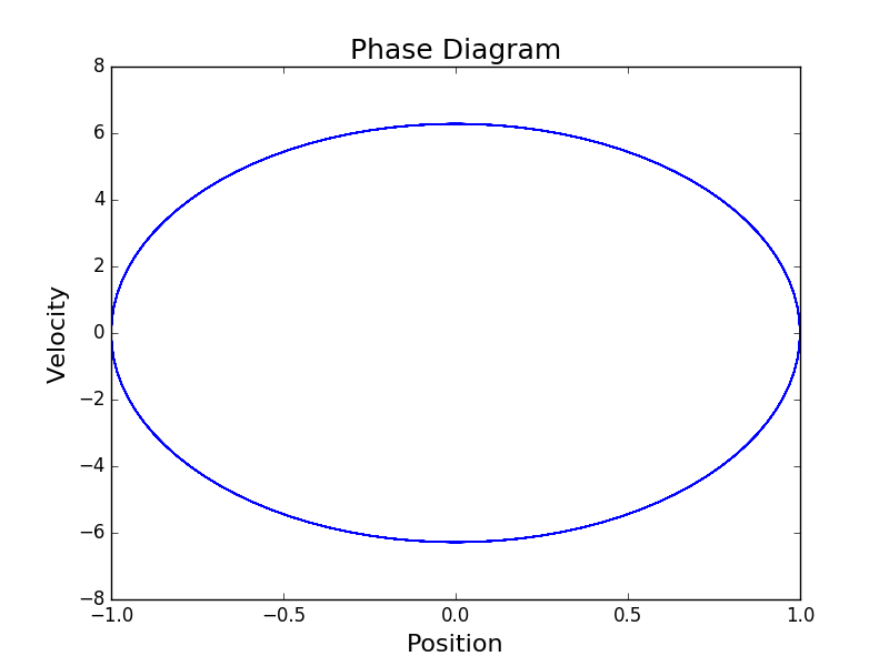
The phase diagram will become an important part of our error analyses. Since we have an analytical solution, we can compute the errors in the positions and velocities resulting from the numerical integration. Beyond local and global error analysis, MD requires that integrators are symplectic, or volume preserving in phase space, in order to ensure conservation of energy. The phase diagrams will give us a nice visual way of confirming that property.
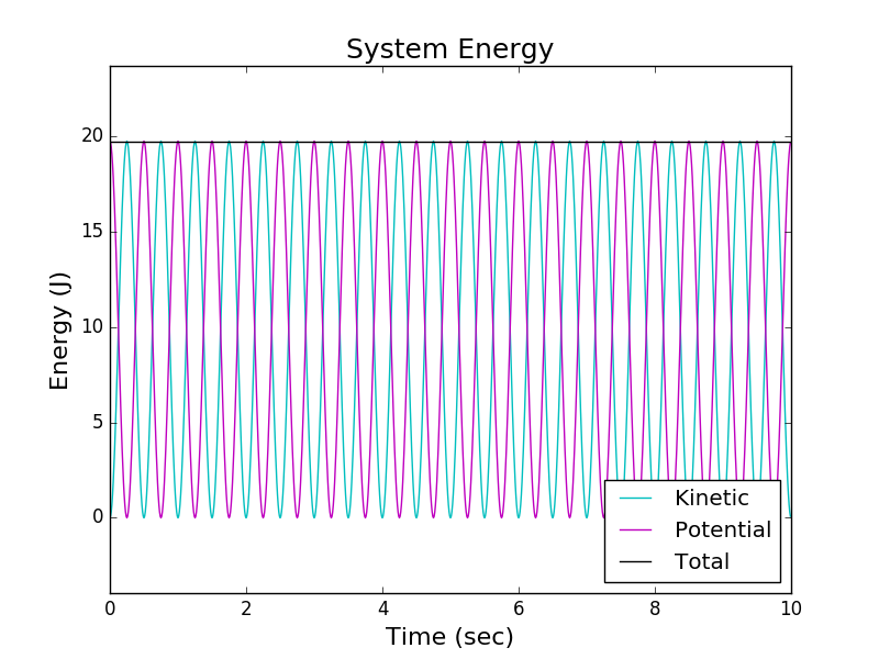
I also computed the potential and kinetic energies at each timestep. The kinetic energy is given as
\[E_K = \frac{1}{2} m v^2\]and the total energy is:
\[E_T = E_K(v) + U(x)\]for some fixed \(E_T\).
If we plot the kinetic, potential, and total energy, we can see that the total energy (black) is conserved, but is transformed transformed between kinetic (cyan) and potential (magenta) energy over time:
In MD, it is also common to evaluate integrators by measuring the error in the energies. I’ll explore that further in a future blog post.
For now, I’ve walked through the basic harmonic oscillator model. I’ve discussed some of the physical choices made for the dynamics of the model. And lastly, I briefly explored two properties of the model.