Verifying Global Error of the Leapfrog Integrator
In my last blog post, I described how to derive the local truncation, or per-step, error analytically. I then compared the analytical prediction to empirical results from the harmonic oscillator model I described in another previous blog post. In this blog post, I’ll derive the global truncation error, or the error accumulated over all of the steps in a trajectory, and once again, compare to the error calculated from harmonic oscillator model.
In our last blog post, we found the local truncation error \(e_{t+\Delta}\) for step \(t + \Delta t\) is given by:
\[e_{t+\Delta t} = \frac{1}{6} \Delta t^3 |x'''(t)|\]We can make the assumption that the errors accumulate linearly, meaning that the global truncation error over some time period \(\hat{t}\) is bounded by the sum of the local truncation errors of the \(N\) steps in the trajectory1:
\[|E_{\hat{t}}| \leq \sum_{i=1}^N \Delta t^3 \frac{|x'''(i \Delta t)|}{6}\]Further, we can assume that the local truncation error of each step is bounded by the maximum local truncation error (with time \(t^*\)) of all steps:
\[\DeclareMathOperator*{\argmax}{arg\,max} t^* = \argmax_{t \, \leq \, \hat{t}} |x'''(t)| \\ e_{i \Delta t} \leq e_{t^*} \text{ for all } 1 \leq i \leq N\]Thus, we can simplify our bound on the global truncation error to:
\[|E_{\hat{t}}| \leq N\Delta t^3 \frac{|x'''(t^*)|}{6} \\\]We note that the time elapsed comes from taking \(N\) steps of length \(\Delta t\):
\[\hat{t} = N \Delta t \\ N = \frac{\hat{t}}{\Delta t}\]By substituting for \(N\), we get our final expression of the bound:
\[|E_{\hat{t}}| \leq \hat{t}\Delta t^2 \frac{|x'''(t^*)|}{6}\]Numerical Experiments
Using a harmonic oscillator model solved with the analytical and Leapfrog methods, we can demonstrate how to verify the per-step error. We note that the global truncation error is dependent on two variables: the timestep \(\Delta t\) and the elapsed time \(\hat{t}\). We will start by evaluating the scaling of \(E_{\hat{t}}\) with respect to \(\hat{t}\) by holding \(\Delta t\) steady.
Using the leapfrog method, we simulated the harmonic oscillator model over 100 seconds using a timestep of \(\Delta t = 0.01\) seconds. We also calculated the positions and velocities using the analytical model at each timestep. We then calculated the global truncation error by subtracting the leapfrog-calculated position and velocity for each step from the analytical position and velocity, respectively.
Since our analytical approach gives us an upperbound on the global truncation error, we found the maximum error for each timestep \(t\) as the maximum of the errors for that and every prior timestep. We then verified that the maximum error scales linearly with the elapsed time by fitting the following equation with linear regression to find values for \(m\) and \(b\):
\[\max_{t \leq \hat{t}} |E_{\hat{t}}| = m\hat{t} + b\]The global truncation errors of the positions and velocites are plotted in the following graphs:
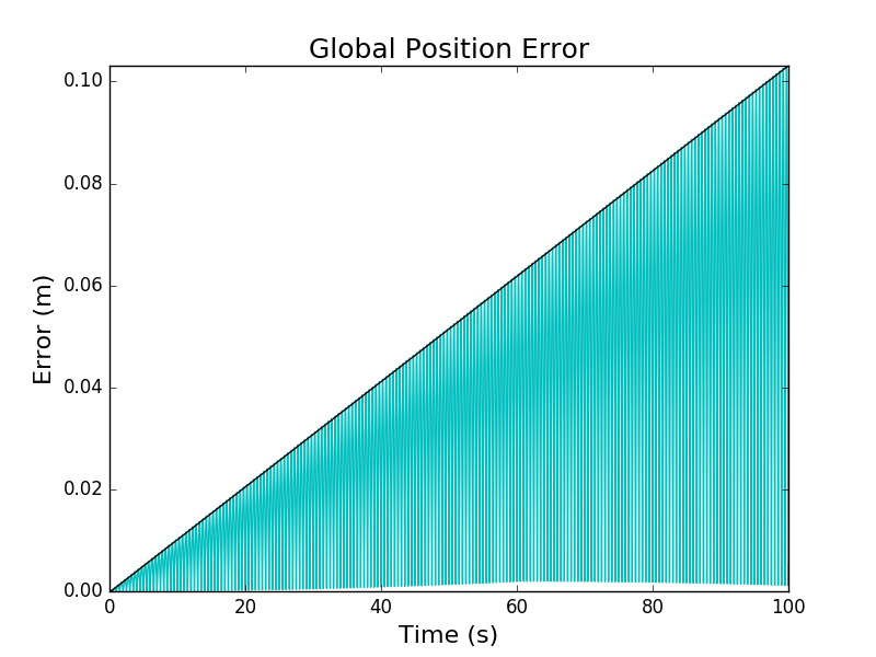
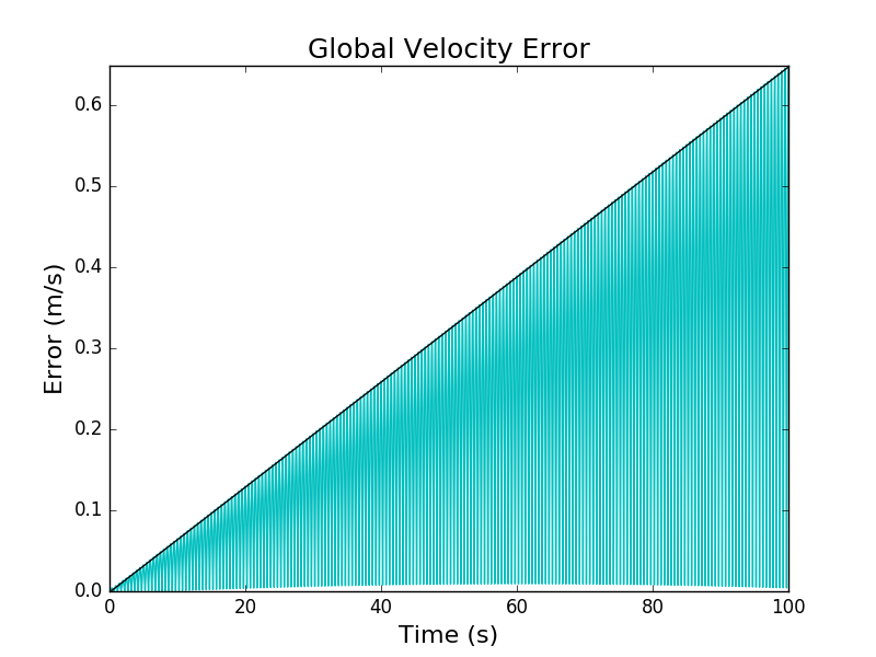
The cyan lines are the global truncation errors accumulated over time, while the black curves correspond to the lines fitted to the maximum global truncation errors as a function of elapsed time. We can see that the fitted lines approximate the maximums well. This is confirmed by \(r^2\) values of 0.999977182194 for the positions and 0.999976016476 for the velocities. Thus, we can be confident that the linear scaling of the global truncation error with respect to the elapsed predicted by our analysis holds empirically.
We notice that the global truncation error oscillates from step to step. In particular, the global truncation error seems to following a periodic function with an amplitude that grows linearly. For the harmonic oscillator model, we can actually calculate the global truncation error exactly.
First, we note that the third derivative of the analytical harmonic oscillator model is given by:
\[x'''(t) = A m \omega^3 \sin(\omega t + \phi)\]Thus, the global truncation error for the harmonic oscillator model is given by:
\[|E_{\hat{t}}| \leq \frac{\hat{t}\Delta t^2}{6} |A m \omega^3 \sin(\omega \hat{t} + \phi)|\]The \(\sin(\omega \hat{t} + \phi)\) term explains the periodic behavior we observed, while the \(\hat{t}\) coefficient explains the linear scaling of the amplitudes we observed.
Next, we empirically validated the order of the scaling of \(E_{\hat{t}}\) with respect to the time step \(\Delta t\). We ran simulations of the harmonic oscillator model for 100 seconds, but with a range of timesteps and number of steps. We found the maximum global truncation error for the positions and velocities from each simulation. The resulting data is reproduced here:
| Step size | Steps | Max Position Error | Max Velocity Error |
|---|---|---|---|
| 0.1 | 1000 | 0.02623153722 | 11.94019129 |
| 0.05 | 2000 | 1.925578275 | 12.03171521 |
| 0.025 | 4000 | 0.6346311748 | 3.990773601 |
| 0.01 | 10000 | 0.1030791043 | 0.6491622412 |
| 0.005 | 20000 | 0.02577397522 | 0.1623304312 |
| 0.0025 | 40000 | 0.006443626148 | 0.04058671379 |
| 0.001 | 100000 | 0.001030963096 | 0.006493957821 |
We then estimated the order of the error with respect to the timestep. Assume the max error is dominated by the time step to a power. We set up an equation to model that relationship and took the logarithm of both sides:
\[|E_{\hat{t}}| \leq c \hat{t} \Delta t^n \\ \log |E_{\hat{t}}| = \log c \hat{t} \Delta t^n \\ \log |E_{\hat{t}}| = \log \Delta t^n + \log c \hat{t} \\ \log |E_{\hat{t}}| = n \log \Delta t + \log c \hat{t}\]where \(E_{\hat{t}}\) is the maximum accumulated error, \(\Delta t\) is the time step, \(n\) is the order, and \(c\) is a constant.
Using the log-log formulation, we then estimate \(n\) and \(c\) using linear regression on the table of time steps and average errors. Our initial results were off. When we plotted the log-log lines, we saw that the model fit well for timesteps \(\leq 0.025\) but not the two larger timesteps. We re-calculated the linear regression excluding the two largest timesteps.
| Error Type | Estimated Order | \(r^2\) |
|---|---|---|
| Position | 1.99599570395 | 0.999996506915 |
| Velocity | 1.99553638001 | 0.999995809409 |
The global truncation errors for the positions and predictions from the log-log model are graphed below:
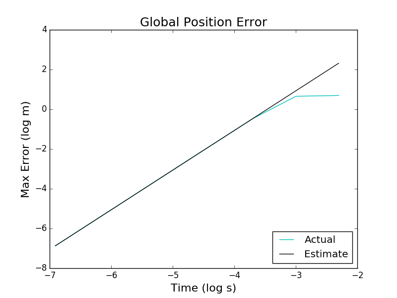
We can see that the maximum global position and velocity truncation errors scale approximately quadratically with respect to the timestep, matching our expectation from the analytical analysis.
(All code for this blog post is available on GitHub under the Apache License v2.)
Conclusion
In this post, we showed how to analytically derive an upperbound for the global truncation error2. We then validated that the maximum global truncation error scales linearly with the elapsed time and quadratically with the timestep using the harmonic oscillator model.
In our numerical experiments, we observed that the global truncation error oscillates periodically with the amplitude growing linearly. We then derived the exact upperbound of the global truncation error for the harmonic oscillator, which confirmed our observations.
Our numerical experiments also demonstrated that the analytical derivation of the upperbound on the global truncation error is not valid for large timesteps. The error for the larger timestep is probably affected by linear or nonlinear instabilities, which we will explore in a later blog post.
1: I used chapter 8 of Elementary Differential Equations and Boundary Value Problems by Boyce and DiPrima as a reference for how to calculate the error.
2: Our derivation matches reported error analysis for the Leapfrog method in Integration Methods for Molecular Dynamics by Leimkuhler, Reich, and Skeel. The authors do not give their derivation, however.