Symplectic Integrators Bound Energy Error
In my previous blog posts, I analyzed the position and velocity error of the harmonic oscillator simulated with the Leapfrog integrator. I proved that the Leapfrog integrator is a second-order method. Using a simulation, I validated that the error of the positions and velocities between the numerically-integrated and analytical models grows linearly with the trajectory length and quadratically with the timestep.
What about the error of the total energy between the numerically-integrated and analytical models? The total energy $E(t)$ is calculated from the positions \(x(t)\) and velocities \(v(t)\) by
\[E(t) = \frac{1}{2}m v^2(t) + \frac{1}{2} m \omega x^2(t)\]As the errors in the positions and velocities grow linearly with time, we can write the numerical positions and velocities as pertubations of the true positions and velocities:
\[\tilde{x}(t) = x(t) + \mathcal{O}(t) \\ \tilde{v}(t) = v(t) + \mathcal{O}(t)\]We can then substitute the perturbed positions and velocities into \(E(t)\) to get \(\tilde{E}(t)\) and solve:
\[\tilde{E}(t) = \frac{1}{2}m \tilde{v}(t)^2 + \frac{1}{2} m \omega \tilde{x}(t)^2 \\ \tilde{E}(t) = \frac{1}{2}m (v(t) + \mathcal{O}(t))^2 + \frac{1}{2} m \omega (x(t) + \mathcal{O}(t))^2 \\ \tilde{E}(t) = \frac{1}{2}m (v(t)^2 + \mathcal{O}(v(t)t) + \mathcal{O}(t^2)) + \frac{1}{2} m \omega (x(t)^2 + \mathcal{O}(x(t)t) + \mathcal{O}(t^2)) \\ \tilde{E}(t) = \frac{1}{2}m v^2(t) + \frac{1}{2} m \omega x^2(t) + \mathcal{O}(v(t)t) + \mathcal{O}(t^2) + \mathcal{O}(x(t)t) + \mathcal{O}(t^2) \\ \tilde{E}(t) = \frac{1}{2}m v^2(t) + \frac{1}{2} m \omega x^2(t) + \mathcal{O}(t^2)\]For the harmonic oscillator, the positions and velocities are bounded by constants. Thus, we end up with linear and quadratic error terms depending on \(t\). Since the quadratic error term to be the largest term in the large \(t\) limit, we can expect the error in the energies be bounded by quadratic growth with respect to the length of the trajectories.
Let’s do a simulation to validate our result. I simulated the harmonic oscillator using the Leapfrog integrator with a timestep of 0.01 s to generate trajectories ranging from 1 s to 1000 s. I sampled the total energy at each time step and plotted the average and standard deviations of the energies (black) for each trajectory length. I also included the analytical energy (magenta) as a reference.
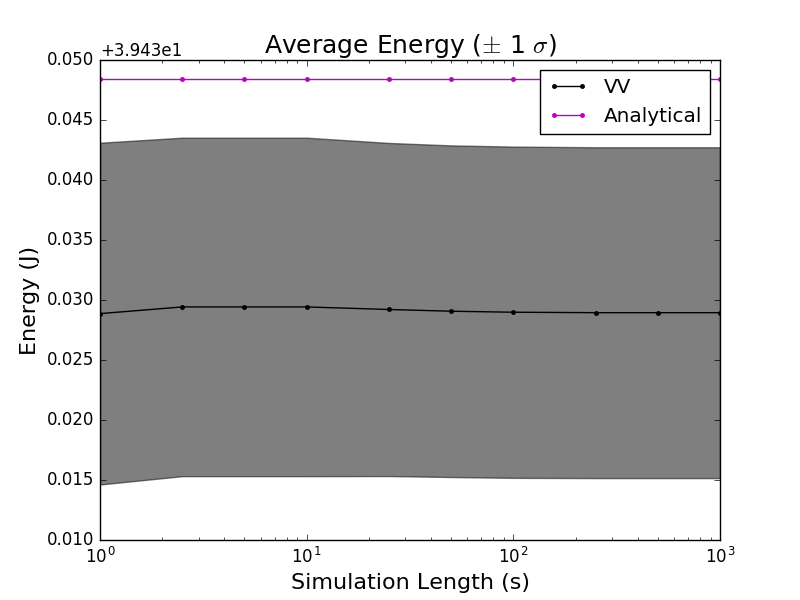
But wait! The energy doesn’t grow over time! In fact, the error in the energy doesn’t seem to change in time once the trajectories are long enough. What’s going on?
Our analysis above provided an upper-bound on the energy error over time – the error in the energy could always be less. Specifically, we didn’t take into account the stricter property of symplectiness.
In my last blog post, I proved that the Leapfrog integrator is symplectic. Ge and Mardsen proved that if a symplectic integrator exactly conserves the total energy (Hamiltonian) of a system, then it is computing the exact trajectory for that system. They go on to suggest that for symplectic integrators, the error in the energy is a good proxy for evaluating the error in the trajectory.
Specifically, symplectic integrators seem to bound the error in the energy so that it doesn’t grow over time. Physicists would say that the error is secular. This is a useful property when studying physical systems.