In my last blog post, I compared several options for Logistic Regression applied to the problem of spam classification. In text classification and other problems, we need to create a mapping from words parsed from the documents to an index in the feature vectors. A common approach for doing this is to extract a vocabulary from the set of training documents and assign an index to each word in the vocabulary. The major advantage of this approach is that it makes it easy to do a reverse mapping from feature vectors indices back to words; this reverse mapping can be particularly useful if you want to analyze which features are most predictive in a model.

There are two primary downsides to vocabulary extraction and indexing as well. First, we need to extract the vocabulary before we can vectorize any of the documents. If the training set can’t fit into memory, this means two passes over the data. For distributed computing environments, this also means the (rather large) vocabulary needs to synchronized across nodes.

Secondly, we can’t easily update the vocabulary as we see new documents. Consider a use case where you use online learning to periodically update a model. You may not want to completely retrain the model from scratch but rather, due to performance considerations, you want to make in-flight updates as additional training data becomes available. If those new documents have previously unseen words, you have two choices. The easiest approach is to simply ignore the new words, but this limits the online learning ability of your model. Secondly, you could reserve empty features to be used for new words and update the feature map as new words are encountered, but maintaining such a large amount of mutable state can be challenging from an engineering perspective.

An alternative is feature hashing, or the hashing trick. With feature hashing, we use the hash of the words to index into the feature vector. With feature hashing, we don’t need to construct or update a vocabulary and accompanying map to feature indices. This makes online learning easier since we don’t need to make two passes over the training data. In distributed environments, we don’t have to perform any synchronization. And if a new word is encountered, the new word gets mapped automatically to an existing feature.

Feature hashing has downsides, too, of course. It isn’t easy to do a reverse mapping from features to the vocabulary; feature hashing can limit the ability to perform introspection on your model.

The number of features is also a parameter now. Whereas we previously knew the number of features from the size of the vocabulary, we now have to explicitly choose the number of features. If we choose too few features, collisions where multiple words are mapped to the same indexed can occur. If we choose too many features, we waste memory since a majority of the features are likely to have values of zero.

In this blog post, I want to compare feature hashing to vocabulary extraction and indexing in terms of accuracy and model size. Scikit-learn offers a HashingVectorizer which makes it easy to experiment with feature hashing.

As before, I used the publicly available trec07p spam classification dataset. I used Python’s built-in email.Parser implementation to extract the email bodies and BeautifulSoup to extract the text. I reserved the first 75% of the 75,419 emails for training and the remaining 25% for testing. I configured the HashingVectorizer to output binary features with no normalization. (IDF scaling isn’t an option.) I used the SGDClassifier to train a Logistic Regression model with log loss penalty and L2 regularization.

For comparison, I also trained a model using the TfidfVectorizer. I set up the vectorizer to output binary features (whether or not a word is present) with no normalization or inverse document frequency (IDF) scaling.

To evaluate the effect on accuracy and collisions, I swept over the number of features, training and evaluating a model for each value. I evaluated accuracy by calculating the area under the (ROC) curve with the test set. I evaluated collisions by calculating the number of features with non-zero weights in the model. If a feature is unused, the model will have a zero weight. If collisions occur, then the number of features with non-zero weights will be less than in a model with no or fewer collisions.

Here are the resulting curves:

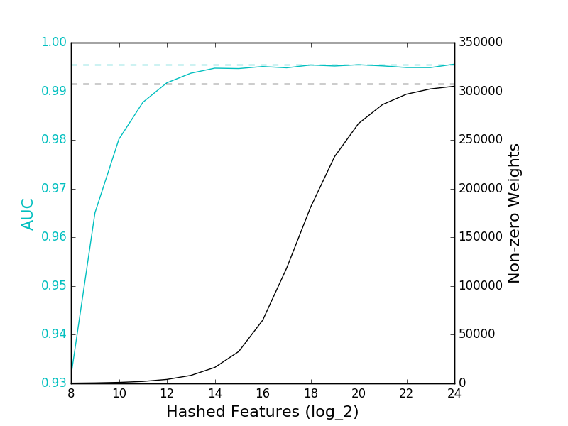
The solid cyan line refers to the AUC of the featured hashing models, while the dashed cyan line is the AUC of the TFIDF model. The solid black line gives the number of features with non-zero weights in the feature hashed models, while the dashed black line gives the number of features from the TFIDF model.

We can make a few observations:

1. The feature hashing model is able to achieve a comparable AUC score to the TFIDF model.
2. The feature hashing model only requires 2^16, or 65,536, features, compared to 307,969 features of the TFIDF model. (Note that I didn’t filter out infrequently-appearing features from the TFIDF model – it’s possible that the size of the TFIDF model could be reduced without significantly affecting accuracy.)
3. We need 2^24, or 16,777,216, features in the feature hashing model to avoid a significant number of collisions. This is a significantly larger number of features than required by the TFIDF model.
4. That said, increasing the number of features beyond 65,536 didn’t seem to improve accuracy so number of collisions is a very conservative metric and shouldn’t be the sole metric used for determining the number of features.

Conclusion

Feature hashing offers some nice advantages, especially for online learning and distributed computing. We observe that with feature hashing we can achieve comparable accuracy to models without feature hashing. The feature hashing models do not seem to require as many features to achieve comparable accuracy, but require many more features to prevent collisions.

(You can download the script I used for this experiment and try it for yourself.)