Pitfalls When Working With Imbalanced Data Sets
I recently started a new job as a data science engineer at an adtech company. Such companies need to train models on massive amounts of data and be able to predict within the time it takes for a web page to load whether or not a user will click on a given ad.
Given these requirements, Logistic Regression (LR) is a popular technology choice for building models. LR models can be quickly trained on huge numbers of data points with many features in a fairly short period of time. When combined with techniques such as stochastic gradient descent, LR can support online learning and very sparse data sets. LR is one of the few modeling techniques which can not only predict probabilities in addition to discrete classes but reasonably accurately, too. And crucially, LR models can be used to serve predictions with very low latencies – evaluating a model requires calculating barely more than a dot product!
I wanted to get some quick hands-on experience with LR models, so I turned to two of my favorites: scikit-learn and the book Doing Data Science. Chapter 5 of Doing Data Science actually describes how adtech company Media 6 Degrees (now called dstillery) uses LR to predict which users will click on an ad and provides an example dataset. Great!
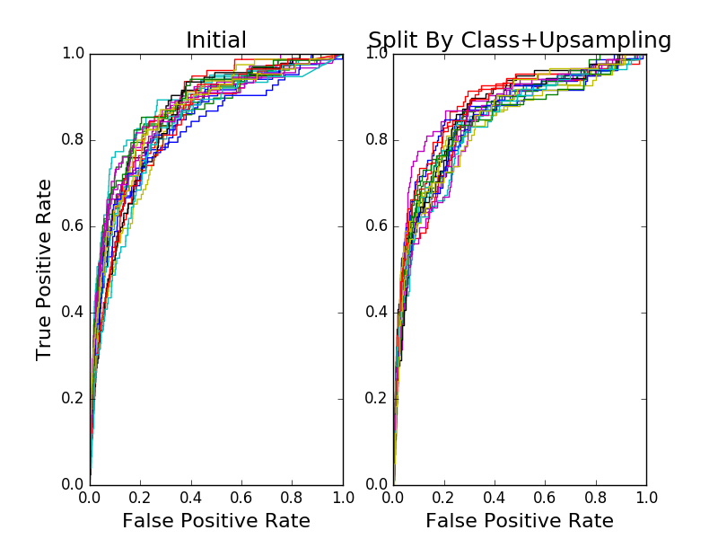
I knew the dataset was imbalanced – after all, most users rarely click on ads. Of the 54,584 entries in the dataset, only 253 are for users with clicks – the remaining users fell into the “no click” class. I decided to just go ahead and train a LR model since I would be experimenting with techniques to improve it’s performance anyway. I used scikit-learn’s built-in split function to randonly allocate 67% of the data points to training and the remaining 33% to testing. I built 20 models, each with a different split. And, I evaluated the resulting models using ROC curves, area under the (ROC) curve, and log loss.
I then decided to tackle the class imbalance. I wrote my own split function to divide the data points by class, perform the random split within each class, and merge the results. This way, the class proportions would be maintained, and I wouldn’t be accidentally sampling data points only from the majority class. I also upsampled the minority class to compensate for the imblance. I trained 20 models and evaluated them using the same metrics as before.
This is what I got:
| Metric | Initial Model | Split By Class + Upsampled Model |
|---|---|---|
| Average AUC | 0.855 | 0.854 |
| Std AUC | 0.0176 | 0.0125 |
| Average log loss | 0.0248 | 0.490 |
| Std log loss | 0.002 | 0.023 |
From what I could tell from the ROC curves, the two models were indistinguishable. This made very little sense given my prior experience. Even more confusing, the log loss got worse!
I decided to print out a confusion matrix for a model of each type and that’s when the lightbulb went off:
| Predicted No-Click | Predicted Click | |
|---|---|---|
| No-Click | 100% | 0% |
| Click | 100% | 0% |
| Predicted No-Click | Predicted Click | |
|---|---|---|
| No-Click | 84.4% | 15.6% |
| Click | 30.1% | 69.9% |
I was using the wrong metrics. The ROC curves and area under the curve scores use the predicted probabilities, not the predicted class labels. The models are likely producing probabilities of different magnitudes but of consistent ordering. Since the decision function is probably centered around 0.5, the probabilities from the first model are resulting in different class predictions than those from the second model. This is an example of why you should be careful about using a default decision function and even consider approaches like probability calibration.
On the other hand, the log loss metric does use the class predictions from the decision function, but weights each type of misclassification equally. Because there are very few click user data points, a model can mispredict all click users as no-click users and still appear to have a small log loss. This is exactly what is happening with the first model. By balancing the composition of the training set, the second model correctly identifies 69.9% of the click users but mispredicts 15.6% of the no-click users as click users, resulting in a larger number of mispredictions and worse log loss. As such, we have to be careful about using log loss when the costs of the type of mispredictions are unequal or the classes are imbalanced.
A few lessons learned:
- Class imbalance significantly impacts logistic regression’s class predictions if you don’t account for the imbalance in the decision function.
- Orderings of data points by the predicted probabilities seem to be consistent even in the face of class imbalance, though. It would be good to follow up on this by comparing rankings using something like Kendall’s Tau.
- ROC curves and AUC seem to be robust to class imbalance.
- Log loss is not robust to class imbalance. I imagine the metric could be generalized to incorporate misprediction costs and adjusted to account for class imbalance, though.
If you want to play with the models yourself, feel free to grab the script I used to generate the figures and metrics.
(While writing this blog post, I came across an excellent blog post titled “Learning from Imbalanced Classes” which gives a great overview of the issues of learning and evaluating with imbalanced datasets and techniques for addressing those issues. It also includes some great illustrations.)