In our previous blog post, we discussed the feature hashing trick and demonstrated its properties and advantages when applied to spam classification. It turns out that the hashing trick can be used in other contexts. In particular, the hashing trick makes it feasible to build a recommendation system from a logistic regression model.

To simplify the problem, we’re going to focus on predicting whether a user will watch a movie based on other movies they’ve watched. Thus, for a given input pair \((u, m)\) of user \(u\) and movie \(m\), we want to predict whether the user will (0) or will not (1) watch the movie. As a logistic regression model can also predict the probability of the interaction in addition to a binary label, we can use the predicted probilities to sort the movies in terms of users and recommend some fixed number of top-ranked movies.

Crafting the Features and Logistic Regression

At first, it may seem very counterintuitive to use Logistic Regression to predict interactions across multiple movies since it only outputs a binary label or single scalar probability. However, we must remember that the model is linear – a sum of terms.

Let’s say that we have \(N\) users, \(M\) movies, and \(K\) features per movie. For each user, we can define a feature vector with \(MK\) entries. When we want to predict interaction for a pair \((u, m)\) of user \(u\) and movie \(m\), only features with indices in \([mK, (m+1)K)\) will be “on” (have non-zero values). The other \(M(K-1)\) features will be set to zero. This enables us to pack \(M\) separate logicistic regression models into a single logistic regression model.

In our case, for each movie \(m\), we’ll use the interactions with the \(M-1\) other movies as the features¹. Thus, \(K=M-1\) and our vector will have \(M(M-1)\) entries. This should immediately raise a concern about memory usage – the number of features will scale quadratically with the number of movies. In fact, this is one reason why you wouldn’t to train a separate model for each movie in the first place anyway.

This is where feature hashing comes to our rescue. The interactions are very sparse; a small percentage of the \(M-1\) features for each movie are likely to be on. Instead of having a vector of \(M(M-1)\) entries for each user-movie pair \((u, m)\), we can create a small vector of \(2^B\) entries (where \(B\) is a new parameter for the model). For each movie \(i\neq m\) that the user has watched, we can encode the ids \(m\) and \(i\) as a string \(s\) (e.g., 23432_768). By hashing the string, we can find the index in the feature vector idx = hash(s) % 2**B and increment the count at that index.

As with most of our blog posts, we implemented a proof of concept using the wonderful scikit-learn. We used the SGDClassifier with a L2 penalty and log loss. Features for each user-movie pair were hashed with the FeatureHasher extractor. The model was trained in an online fashion, with each a batch formed for each user from the user’s positive and negative examples. We released the implementation on GitHub under the Apache v2 License.

Evaluation

Training and Test Sets

We tested the approach using the MovieLens 10M dataset. We binarized the user-movie ratings matrix to produce an interaction matrix. We randomly chose 1000 users without replacement for training and another 100 users for testing. For each user, we created data point with a positive label (1) and corresponding feature vector for each movie seen and an equal number of data points with negative labels (0) and corresponding feature vectors by randomly sampling without replacement from the movies the user hadn’t seen. Thus, each positive training or test example had a corresponding negative example (no class imbalance).

Model Parameters and Accuracy

We evaluated accuracy by computing the area under the ROC curve from the true labels and predicted probabilities. The only free parameter is \(B\), \(\log_2\) of the number of entries in the feature vector model. We plotted the model AUC and number of non-zero features for multiple values of \(B\) to ascertain the number of hashed features needed for accuracy to plateau.

Here are the resulting curves:

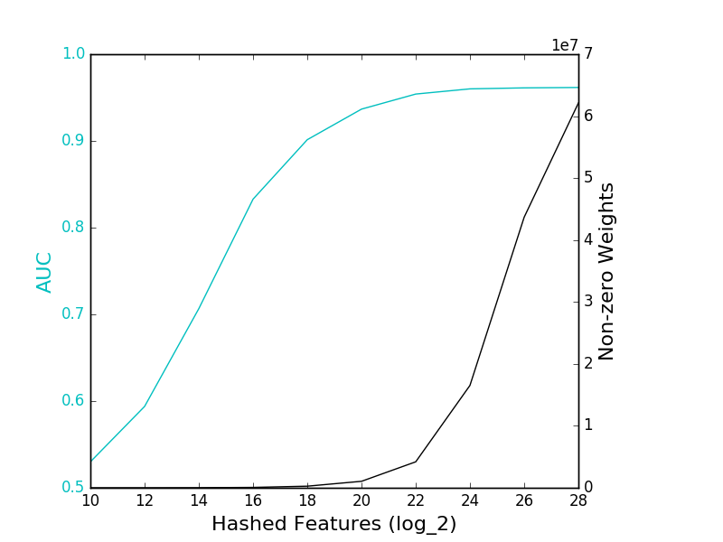
The solid cyan line refers to the AUC of the featured hashing models, while the solid black line gives the number of features with non-zero weights in the models.

The model achieved a maximum AUC of 96%, which is quite respectable for such a basic model. Accuracy plateaus at around \(2^{24}\) entries continues to improve up to \(2^{28}\) entries, suggesting that higher AUCs may achievable with larger models, but the difference is likely to be small.

Conclusion

In this post, we explained how to build a model for predicting user interactions with products using Logistic Regression. We demonstrated how multiple conceptual models can be packed into a single model instance by properly encoding the features. We also demonstrated how feature hashing can be used to reduce the quadratic scaling of the features to a more manageable size. Lastly, we evaluated the accuracy of the model on the MovieLens dataset, achieving an AUC of 96% when using \(2^{28}\) hashed features.

The disadvantage of this approach is the number of evaluations required to find a list of top recommendations across all products. To find the top-ranked products for a user among all products, we would have to generate features and evaluate every the model for every product. For large retailers will millions of users and products, this brute-force approach is simply infeasible.

The simplest way to reduce the number of evaluations would be to reduce the number of products to evaluate. Ever notice that Amazon and Netflix break their recommendations down by into subcategories and genres, respectively? For example, for me, Amazon tends to offer recommendations for math and history books and science fiction books and TV shows. We could limit our evaluations to the top, say, 10,000 products in categories that user has browsed.

In fact, the ability to evaluate on only a desired subset of products can be an advantage. Since the model is trained on the global space of product interactions, the model can incorporate interactions between products in different categories such as history books and TV shows. When we go to recommend products, however, we can easily limit our predictions to a particular type of product.

1: We do not include an interaction feature for the movie in the user-movie pair for which we are trying to predict an interaction. The feature would always be on for positive training examples and off for negative training examples, leading to perfect correlation with the output label. This would lead to overfitting and poor accuracy in testing. Hence, why we have \(M-1\) features per movie.